How Do RAG Systems Search? HNSW

With the boom of artificial intelligence, different techniques for retrieving information have become popular, such as RAG. We are going to look at an algorithm that works underneath when it comes to using embeddings.

This time we will not talk about how those embeddings (vectors) are generated, but rather how they are searched quickly and efficiently.

What Is a Vector?

Remembering a little bit of mathematics, a vector can be understood as an element that has direction and magnitude.

In a three-dimensional space, it can be represented as follows:

$\vec{v} = \langle x, y, z \rangle$

Each component represents the magnitude of the vector along one of the axes.

Embeddings are vectors, but with many more dimensions. They can semantically represent text, images, etc.

How Is Similarity Between Vectors Calculated?

One of the most commonly used metrics is cosine similarity.

To understand it, let’s first remember the dot product. Given the following vectors:

$\vec{u} = \langle u_x, u_y, u_z \rangle$ and $\vec{v} = \langle v_x, v_y, v_z \rangle$

The dot product can be calculated using their components:

$\vec{u} \cdot \vec{v} = u_xv_x + u_yv_y + u_zv_z$

It can also be defined based on the angle that exists between both vectors:

$\vec{u} \cdot \vec{v} = \lVert\vec{u}\rVert \lVert\vec{v}\rVert \cos(\theta)$

Where:

• $\lVert\vec{u}\rVert$ is the magnitude of $\vec{u}$.

• $\lVert\vec{v}\rVert$ is the magnitude of $\vec{v}$.

• $\theta$ is the angle between both vectors.

If we solve for $\cos(\theta)$, we get the cosine similarity formula:

$\text{Cosine Similarity} = \cos(\theta) = \frac{\vec{u} \cdot \vec{v}}{\lVert\vec{u}\rVert \lVert\vec{v}\rVert}$

The result tells us how aligned the vectors are:

• A value close to 1 indicates high similarity.

• A value close to 0 indicates little relationship.

• A value close to -1 indicates opposite directions.

A small optimization is to normalize the vectors beforehand so that they have a magnitude equal to 1:

$\lVert\vec{u}\rVert = 1 \quad \text{and} \quad \lVert\vec{v}\rVert = 1$

In that case, the formula is considerably simplified:

$\text{Cosine Similarity} = \frac{\vec{u} \cdot \vec{v}}{1 \times 1} = \vec{u} \cdot \vec{v}$

Therefore, when the vectors are normalized, calculating cosine similarity is equivalent to calculating their dot product.

How Does This Apply to Embeddings?

Let’s suppose that the following vector represents a query related to the concept of a “dog”:

$\vec{q} = \langle 0.1, 0.3, 0.2 \rangle$

In a real system it would have many more dimensions, but for practical purposes we will use 3.

If we want to find documents related to dogs, we can generate the embedding of the query and compare it with the embeddings stored in our database.

The simplest solution would be to calculate the cosine similarity between $\vec{q}$ and each of the stored vectors.

However, this means going through the entire dataset.

For n vectors with d dimensions, the approximate cost would be:

$O(n \cdot d)$

If we consider that the number of dimensions is constant, we can simplify it as:

$O(n)$

If we have 100 vectors, performing 100 comparisons does not represent a big problem.

But what happens when we have millions of vectors and thousands of requests per second?

Performing a full scan on every search stops being a practical solution.

This is where approximate nearest neighbor search algorithms, known as ANN, for Approximate Nearest Neighbors, come in.

One of the most popular algorithms for solving this problem is HNSW.

What Is HNSW?

HNSW stands for Hierarchical Navigable Small World.

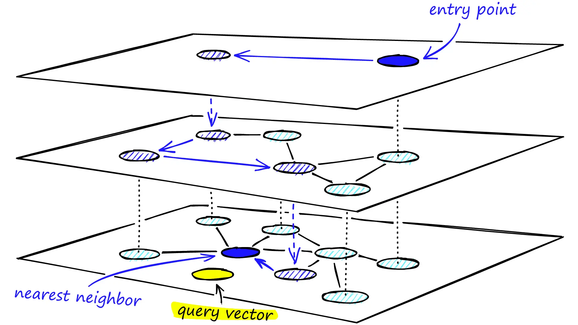
The general idea is to organize the vectors inside a graph composed of different layers or levels.

• The upper layers contain few nodes and allow us to make large jumps.

• The lower layers progressively contain more nodes.

• Layer 0 contains all the stored vectors.

We can imagine this structure as a road network:

• The upper layers work like highways that allow us to quickly get closer to a region.

• The lower layers work like local streets that help us find a more precise location within the selected region.

How Is a New Vector Inserted?

When a new vector is added to the index, the first step is to randomly choose the maximum level in which it will participate.

A simplified implementation could use the following expression:

level = int(-np.log(np.random.uniform(0, 1)) * mL)

Where:

mL = 1 / np.log(M)

Mathematically, we can represent it as:

$\text{level} = \left\lfloor -\log(U) \cdot m_L \right\rfloor$

Where:

$m_L = \frac{1}{\log(M)}$

This distribution makes most nodes remain in the lower layers, and fewer and fewer nodes appear in the upper layers.

Once the level has been selected, the insertion process begins:

1. The search starts from the entry point of the highest layer.

2. At each layer, we navigate toward the node closest to the new vector.

3. When no better neighbor can be found, the search moves down to the next level.

4. In the layers where the new node will participate, a set of nearby neighbors is selected.

5. Connections are created between the new node and the selected neighbors.

6. The process continues until reaching layer 0.

The node is not “cloned” at each layer. In reality, the same node participates in all the layers between its maximum level and layer 0.

This way, all vectors are present in the bottom layer, while only a portion of them work as shortcuts in the upper layers.

How Is a Search Performed?

A query uses a process similar to insertion:

1. The search begins at the highest layer.

2. We calculate which neighbor is most similar to the query vector.

3. The search moves toward that neighbor.

4. The process continues while better neighbors are found.

5. When there is no better option, we move down to the next layer.

6. At layer 0, a larger set of candidates is explored.

7. Finally, the closest vectors found are returned.

Thanks to this hierarchical structure, HNSW avoids comparing the query against all the stored vectors.

In practice, it usually has behavior close to:

$O(\log n)$

However, this complexity is not a strict guarantee. Performance depends on factors such as the distribution of the data, the number of graph connections, and the parameters used during construction and search.

What Are Its Trade-offs?

HNSW performs an approximate search, so it can find an extremely similar vector but does not guarantee the closest one in the entire dataset, since it is a greedy algorithm. Unlike brute force, which would find the closest one but would have linear complexity.

HNSW sacrifices a small amount of accuracy, normally known as recall, to achieve considerably faster searches. It also requires additional memory to store the graph connections and more work during index construction.

There are three important parameters that allow us to control this trade-off:

• M: approximately defines how many connections each node can maintain.

• efConstruction: controls how many candidates are explored during index construction.

• efSearch: controls how many candidates are explored during a search.

Increasing these values normally improves the probability of finding the nearest neighbors, but also increases memory consumption, construction time, or search latency.

A Way to Understand It

If we only had one dimension, we could sort the values and use a binary search.

HNSW is not exactly a binary search extended to multiple dimensions, but it shares a similar intuition: using a hierarchical structure to quickly discard large regions of the search space.

In other words, it allows us to efficiently navigate vector spaces with hundreds or thousands of dimensions.

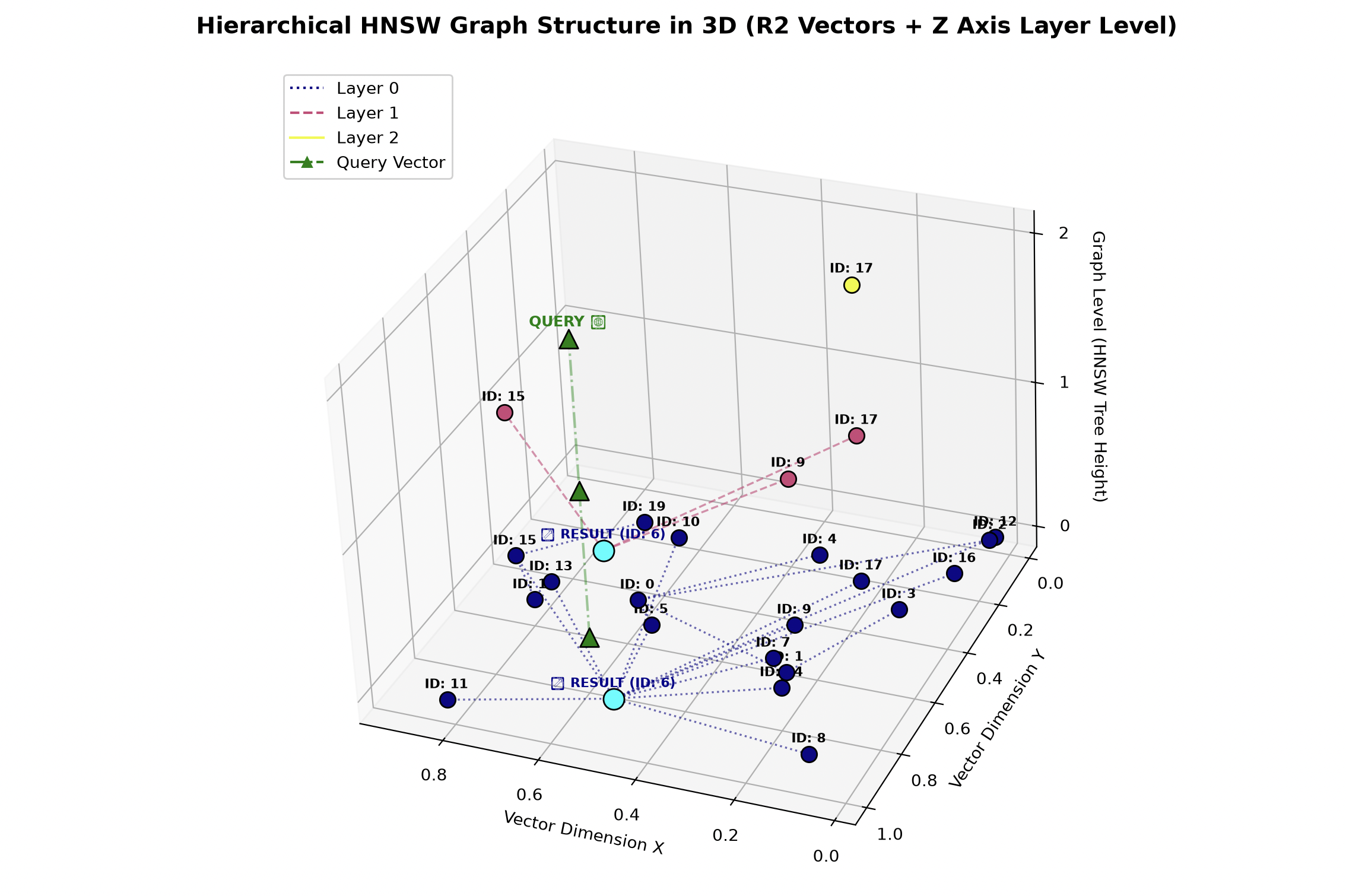
I am also leaving the code on GitHub in case you want to run it, modify its parameters, or visualize how the graph structure changes:

GitHub Code

I hope it helps in some way.